Photo by Rubaitul Azad on Unsplash
How to Use Basic Conditional Formatting in Google Sheets
– Rebekah Hedge
Conditional Formatting is a handy tool in Excel that allows you to change the look of your cell for various reasons.
First: Choose the cell or group of cells that you wish to begin formatting.
Next: Right click and choose “Conditional Formatting.”
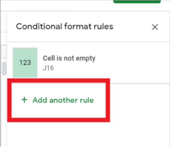
- On the right hand side of the screen the Conditional Formatting box will appear.
- Begin by clicking “Add Rule” as seen below.

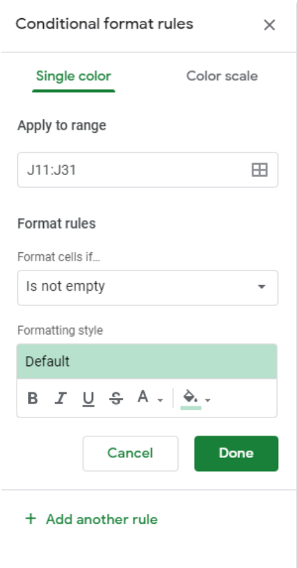
Once you select “Add another rule”, the box below will appear.
- If you have not already chosen the full range of cells that you would like, update the “Apply to Range” field.
- Select the cells you wish to apply the rule
Once you have selected your range, choose the option that you want from the “Format Cells If…” field.
- If the scenario that you want to use to format your cells is not listed, choose “Custom Formula Is.” Doing so will allow you to choose various “=if” formulas.

Next, choose your formatting style. Doing so allows you to update the color, font and other typical formatting of the cells that you have chosen.
- If you choose later to copy this formatting to another group of cells, you can copy the cells and then choose the group of cells, right click and choose “Paste Special”.
- Once these options pop up, choose “Paste Format Only”. This will allow you to copy the formatting through the excel sheet without having to go through all of the previous steps again.
Questions? Contact us via email: [email protected]


